In November, the folks over at Scylla announced that an IoT benchmark of theirs achieved a “1 billion rows per second” scan. In this article I’ll show how you would model this use case differently with Aerospike, in a way that achieves higher performance with less hardware.
Overview
The Scylla benchmark involved 1 million sensors, logging a temperature measurement once a minute for a year, so each sensor logs 1440 measurements per day, 525,600 per year. Last I checked (2019–12–02) this announcement wasn’t published as a detailed benchmark on the Scylla website, but rather as a (2019–11–05) press release, which sketches out their claims. The lack of details is unfortunate, but I’ll work with that.
A Cassandra Modeling Approach
In a Cassandra derivative like ScyllaDB, you would typically have a temperature column containing a single numeric value, with the row representing an instance of measurement. Accordingly, the Scylla benchmark talks about a dataset of 526 billion rows. In this modeling approach, each row is extremely sparse, holding just one data point for a distinct sensor-timestamp pair.
According to the Scylla press release, to retrieve the entire year’s worth of data, you need to scan the dataset. To get 3 months of sensor information you need to scan the dataset. But the same holds for getting a day’s data for all the sensors, a year’s data for a single sensor, or a single day’s data for an individual sensor — you scan the dataset.
Cassandra is a column-oriented database, and as such is more suitable for ad-hoc analytics than key-value operations. Like Aerospike, ScyllaDB is written in C (rather than Java), and Scylla have worked to optimize network and disk IO. The Scylla folks are good engineers, and they’ve put in hard work to be better than Apache Cassandra and DataStax. However, when it comes to transactional workloads (rather than analytics), a row-oriented NoSQL database like Aerospike has the upper hand. Modeling this use case in Aerospike will utilize fewer, larger records, with multiple data points in each.
The ScyllaDB Cluster Capacity
How big is this dataset anyway? Let’s assume that the row’s primary key is (sensor-id , timestamp ) and it has a temperature column with a single int (4B) value. A rough estimate, with a single copy of the data, would be 526 * 10^9 * 16 / 1024^4 = 7.65TiB . The cluster described by Scylla has 83 x n2.xlarge bare-metal servers from Packet.

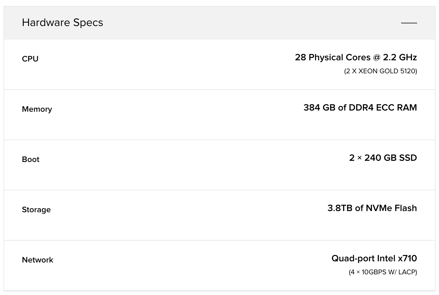
Packet n2.xlarge server specs [2019–12–02]
In total, the cluster has a combined capacity of 286TiB of NVMe Flash, 31TiB of RAM, 2324 physical cores, 3320Gbps of NIC. By my estimate the dataset is 7.65TiB. Yes, the disparity between the cluster capacity and the size of this benchmark’s dataset should raise eyebrows.
An Aerospike Modeling Approach
Data Model
For the same use case described in the overview, we will collect each day’s data from one sensor into a single record. Every minute the application will log a temperature reading as a tuple [timestamp, temperature] and append it to a list of such tuples. At the end of the day this list will have 1440 tuples, and our application will roll over to a new day’s record for the sensor.
The choice of setting the list’s type to UNORDERED versus ORDERED depends on whether we want to optimize for faster writes or faster in-record read operations, such as getting a range of values from the record. The lists’s type does not limit the operations that can be performed, but it does change their performance characteristics. Since time increases monotonically, I’m choosing to use an unordered list, for which the append operation has a O(1) performance.
Storage Requirements
Let’s consider how much space is used for this data structure. Aerospike lists are serialized using MessagePack, which compacts the data. An 8 byte timestamp and an 8 byte float will end up taking 15 bytes.

However, there’s no need to use a full Unix epoch timestamp here. Each record represents a day, so we can instead use midnight as the local epoch and enumerate the minutes since midnight. Midnight would be minute 0, 00:01 would be minute 1, etc. Similarly, the temperature does not need the precision of a float. If the sensor reports temperatures with a precision of one decimal point, we can multiply the value by 10 and store that as a (small) integer. MessagePack can now compact this tuple into 7 bytes.

A reading from 23:22, with a temperature of 62.1 degrees
Leveraging Compression
Compression is an Aerospike Enterprise Edition feature that can be used to further compact the IoT data we are collecting.First, let’s consider the storage requirements without compression. At the end of the day we expect a record to take roughly 10K (1440 measurement tuples, plus some overhead). A year’s data for one sensor is ~ 3.5MB across 365 records. The memory cost for a record is 365 * 64 /1024 = 22.8KiB. In my example, I populated an Aerospike database with a year of measurements from one thousand sensors.

A year of uncompressed data from 1000 sensors in Aerospike Community Edition 4.6
The example above is running on a modest 2 core VM with 16GiB storage allocated and 2GiB of RAM.Next, I upgraded to Aerospike Enterprise Edition 4.7 and added compression to my namespace configuration:
namespace test {
 high-water-disk-pct 80
 high-water-memory-pct 80
 replication-factor 1
 memory-size 2048M
 storage-engine device {
 file /opt/aerospike/data/test.dat
 filesize 16834M
compression zstd
compression-level 1
 }
 }
Compression is applied on a record-by-record basis, so none of the existing data is automatically compressed after restarting the upgraded (EE-4.7) asd. To change this, I wrote a simple UDF that just touches a record, and applied it with a background scan to all the records in my namespace. This caused the records to be updated with a new TTL value, and stored in a compressed state, as defined by the namespace configuration.
Aerospike Query Client
 Version 3.22.0
 C Client Version 4.6.8
 Copyright 2012-2019 Aerospike. All rights reserved.
 aql> register module './ttl.lua'
 OK, 1 module added.
 aql> show modules
 +-----------+--------------------------------------------+-------+
 | filename | hash | type |
 +-----------+--------------------------------------------+-------+
 | "ttl.lua" | "9614a68daf5353109372d96517d3d4f863e64ec1" | "LUA" |
 +-----------+--------------------------------------------+-------+
 [127.0.0.1:3000] 1 row in set (0.002 secs)
 aql> execute ttl.touchttl() on test.sensor_data
OK, Scan job (13120129825472024600) created.
aql> show scans
+----------------+--------+------------+--------------+-------------+--------------+----------------+--------------------+------------------------+--------------+---------------+----------+------------------+--------+----------------+--------------------+------------+----------+--------------+--------+-----------------+----------------+-----------------------+
| active-threads | ns | udf-active | udf-filename | recs-failed | udf-function | recs-succeeded | recs-filtered-bins | trid | job-progress | set | priority | job-type | module | recs-throttled | recs-filtered-meta | status | run-time | net-io-bytes | rps | time-since-done | socket-timeout | from |
+----------------+--------+------------+--------------+-------------+--------------+----------------+--------------------+------------------------+--------------+---------------+----------+------------------+--------+----------------+--------------------+------------+----------+--------------+--------+-----------------+----------------+-----------------------+
| "0" | "test" | "0" | "ttl" | "0" | "touchttl" | "365000" | "0" | "13120129825472024600" | "100.00" | "sensor_data" | "0" | "background-udf" | "scan" | "365000" | "0" | "done(ok)" | "73279" | "30" | "5000" | "1814" | "10000" | "192.168.141.2:54138" |
+----------------+--------+------------+--------------+-------------+--------------+----------------+--------------------+------------------------+--------------+---------------+----------+------------------+--------+----------------+--------------------+------------+----------+--------------+--------+-----------------+----------------+-----------------------+
[127.0.0.1:3000] 1 row in set (0.001 secs)
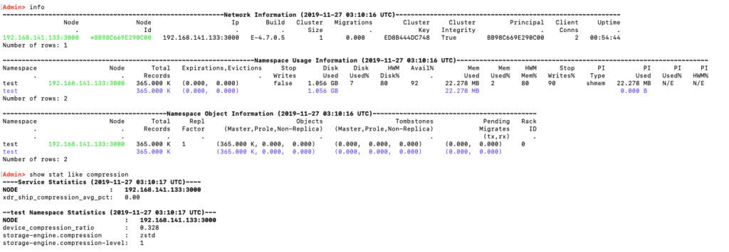
Looking at the cluster with asadm, I saw that the dataset compressed to 32.8% of its original size (device_compression_ratio 0.328).

Same dataset with a 0.328 compression ratio thanks to Zstandard level 1
Compression doesn’t just save on space, it usually also lowers latency, as it’s faster to read a 3KiB object than a 10KiB one, even if the server has to decompress it (zstd has a very high decompression speed compared to the read IO speed).
Code Sample
The code I used is located in the repo aerospike-examples/modeling-iot-sensors. I started by running run_sensors.sh, which launched ten Python populate_sensor_data.py workers at a time, until a few minutes later I had a year of data from a thousand sensors. The sensor data is based on a year of (hourly) temperature data points I had downloaded from NOAA.The query_iot_data.py script has an --interactive mode, which makes it easier to see what it’s doing. Even on my underpowered VM it runs fast over the example data.
To fetch three hours of data from one sensor I used the list get_by_value_interval operation to find all the values between [480, NIL] and [660, NIL]. See the ordering rules for more on how Aerospike compares between values in the list.
Three hours of a single sensor’s data for 2018–12–31
[ [480, 520],
 [481, 521],
 [482, 521],
 :
 :
 [657, 614],
 [658, 614],
 [659, 614]]
Getting a day’s data for any sensor is a single read. The number of records doesn’t matter; the latency of this operation will be the same, regardless of which day we fetch, or how many records are in the dataset.
Gets a single sensor’s data for 2018–04–02
To get a year of data for an individual sensor we do not need to scan the entire dataset. The way we’ve modeled our data allows us to build an array of 365 keys, then use it to make a single batch-read operation. If the batch was bigger it might have been more optimal to iterate through a few sub batches. For information on tuning batch operations see the knowledge base article FAQ — batch index tuning parameters.
Getting the data from all the sensors on a specific day is just as simple. If the batch was bigger than batch-max-requests we would need to either tune that configuration parameter or iterate through several smaller batches.
A day of data from all the sensors, no scan necessary
Finally, we can scan the entire dataset and filter out the records we want using a predicate filter. In the example below, I am doing a modulo operation on the record’s digest. This operation executes on the primary index metadata (in memory), without needing to read the records, so it’s very fast. A predicate filter can be as complex as you need it to be, with the conditional logic applied on the server side.
Scans the entire dataset with a predicate filter, returning about 1000 records
Conclusion
Aerospike is more suited for the type of IoT timeseries data collection and retrieval described in the original benchmark than ScyllaDB. You can intuitively see how with a row-oriented modeling approach, leveraging Aerospike’s strengths, you would get better performance than a C* database, using far less hardware.Aerospike does not yet provide full timeseries database functionality such as being able to apply aggregate functions over a range of data. But it is a high performance, hyper scalable database, and provides the functionality needed for time slicing datasets.
An application can compute its own aggregates over the data retrieved quickly and efficiently from Aerospike. Similarly, you can do such computations in Spark, using Aerospike Connect for Spark to fetch data from Aerospike into Spark. The connector library knows when to use batch reads, and when to scan (with or without a predicate filter), using a similar pattern to my code sample. This approach is already being used in production by enterprise and community users.
Keep reading

Apr 28, 2026
Aerospike Voyager: From first connection to production code

Apr 28, 2026
Introducing the Aerospike Java and Python SDKs: A generational upgrade to building on Aerospike

Apr 22, 2026
Aerospike vs. Cassandra: Databases don’t need to go down to break your application

Apr 16, 2026
Introducing Aerospike 8.1.2: Making nested data queries fast and easy to write
