Making sense of vectors: Why they’re the key to smarter AI searches

Artificial intelligence (AI) is everywhere these days — and for good reason. It’s helping us uncover trends, spot patterns, and solve problems in ways we couldn’t before. From healthcare to retail to research, AI is opening up new possibilities.

But here’s the thing: AI is only as good as the data it has. More data generally means better results, whether you’re training a model, running a similarity search, or using generative AI to form humanly understandable responses. That’s where tools like large language models (LLMs) come in. They’re trained on huge datasets and can generate answers that feel almost human. Pretty amazing, right?

The catch? LLMs don’t always get it right. Without extra context to guide them, they can return answers that are incomplete—or even completely made up, called “hallucinations.” That’s where providing relevant context makes all the difference.

Yet, how do we figure out what context to give these models? That’s where vectors, vector search, and vector databases come in. Unlike traditional keyword searches, vector searches help us zero in on meaning, not just matching words. A vector database stores and retrieves data in a way that’s all about context.

In this post, we’ll break down what vectors actually are, how they work, and why they’re becoming such a big deal for developers building smarter, more reliable generative AI systems.

What is a vector?

Before diving into vector databases and their role in generative AI, let’s start with the basics: what exactly is a vector?

If you search online, you’ll find definitions like these:

A vector is a mathematical approach for expressing and organizing data. The vectorization of data, such as word vectorization, is one of the initial phases in the creation of an ML model. - H20.ai

In artificial intelligence, a vector is a mathematical point that represents data in a format that AI algorithms can understand. Vectors are arrays (or lists) of numbers, with each number representing a specific feature or attribute of the data. - MongoDB

These are accurate, sure—but let’s be honest, they’re not exactly beginner-friendly. After reading those, do you feel like you could confidently explain vectors to someone else? If not, don’t worry. Let’s break it down into something simpler.

A vector is simply an ordered series of numbers. So [1.5, 2.5, 3.0] is an example of a vector, as is [3.0, 1.5, 2.5]. Since the order of the numbers in the vector is important, these two vectors would be considered different, even though they contain the same numbers. One important term is the dimensionality of a vector, which is simply the number of numbers in the vector. Both these sample vectors have a dimensionality of three.

That’s simple enough, right? But it still doesn’t describe why they’re useful or how they’re formed. For illustrative purposes, let’s look at a simple example.

Vector example

Let’s say you’re house hunting. You’ve narrowed it down to a specific suburb, and you know you want a house with about 2,500 square feet (ft²) of floor space and a 6,500ft² lot. In reality, you’d probably have a lot more factors to consider—like the price, number of bedrooms and bathrooms, the age of the house, and whether the kitchen and bathrooms are updated. But for this example, let’s keep it simple and focus only on floor and land area.

To further illustrate vector concepts, assume that floor area is twice as important to you as land area. That means you’re introducing weighting into the equation, giving more importance to one factor over the other.

Since you have narrowed down the region, you discover there are nine properties in the area:

Plotting these on a graph with the desired property marked with a red “x” shows:

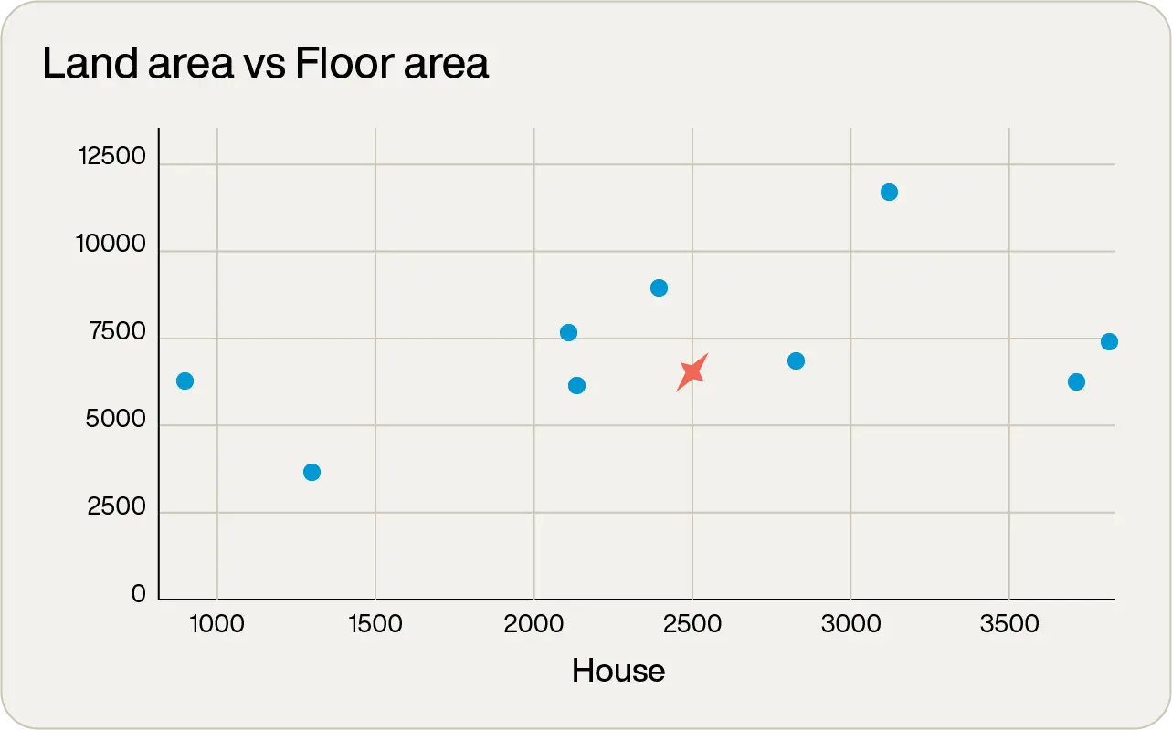
This clearly shows that of the nine properties, four are fairly good contenders. But which one is the “best”?

The two attributes of land area and floor area effectively form a vector with two dimensions. So the first house with a land area of 8,800ft² and 2336ft² floor area would have a vector of [8,800, 2,336], with the first element of the vector being the land area and the second element being the floor area.

The first step is to normalize the vector so each value is in the range from zero to one. This isn’t strictly necessary, but it enables the two dimensions of the vector to be easily compared. Hence, find the largest land area (property 7, 11,780ft²) and divide each land area by this, and do the same with the largest floor area (3,896ft²):

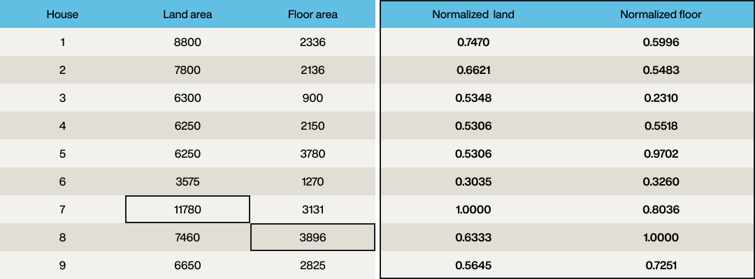
The vector elements are now normalized so that each column has the same range (zero to one). However, the requirement was for the land area to be half as important as the floor area, so to apply the weighting, divide each element of the “land” element of the vector by two:

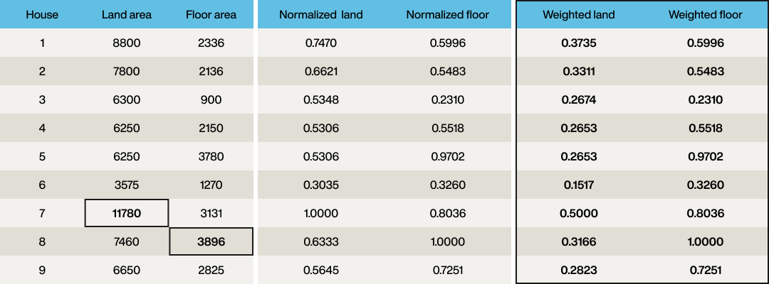
Great! Each property now has a vector that has been normalized. The same process should be applied to the desired requirements. Floor area desired is 2,500ft² so divide this by 3,896 to give 0.6417, and the desired land area is 6,500ft², so divide this by 11,780, then apply the weighting of ½ to give 0.2759. So the query vector is [0.2759, 0.6417].

The process of converting meaningful information into a vector is called embedding. While the example here uses a simple embedding model, real-world scenarios typically rely on more complex systems, like convolutional neural networks (CNNs), which are beyond the scope of this article. However, there are a few key points to keep in mind:

• The vector has no intrinsic meaning in its own right. What does a vector of [0.3735, 0.5996] mean? Since this example is so simple, it could be reverse-engineered to determine the original floor and land areas, but this normally isn’t the case. Vectors are only useful because they are associated with a domain object. Hence, it must be known that that particular vector is associated with property 1 in this case. We will use the term “domain object” to refer to the source object that was embedded to form the vector. This could be structured data, typically a business object like a person, an account and so on, or it could be unstructured data such as text, images, or video.

• The dimensionality of the vector space in this example is just two. This is much smaller than would be used in normal LLM scenarios, which would run from hundreds to thousands (or more) of dimensions.

The embedding model used to embed the nine vectors was exactly the same embedding model used to embed the target data point. This is key – if a different embedding model is used to embed the vectors in the target search space than is used to embed the target point, the results will be meaningless. A consequence of this is that all the vectors produced from the embedding model will have the same number of dimensions.

Vector embedding vs. vector representation

When discussing vector terms in the generative AI space, you will quite often hear the term “vector embedding” or just “embedding.” However, you will sometimes hear the term “vector representation,” which is sometimes used synonymously with vector embedding. But are the two terms the same?

A vector representation is a numerical representation of all the “features” of a domain object that are pertinent to the model. The term feature just represents a single data point, so in our case, the land area is one feature, and the floor area is another feature. 

A vector embedding is the result of applying matrix factorization techniques or deep learning models onto the vector representation to form vectors that are able to be compared with a similarity search.

So, if we consider our first property:

then [8800, 2336] might be considered the vector representation, and [0.3735, 0.5996] would be considered the vector embedding (although with an incredibly simple embedding model!)

Finding the closest vector

Now that all the properties – including the target property – have been encoded as vectors, all that remains is to find the closest vector to the query vector, and that should give the optimal property for our requirements.

This is referred to as a “vector search” or “similarity search.” It is different from searches in traditional databases as it is looking for approximate matches rather than exact matches. What you want is the closest vector(s) from the search set to your reference vector.

But what does “closest” mean?

Euclidean distance

The most intuitive definition of distance is the so-called Euclidean distance, which is what you would get if you measured the distances with a ruler.

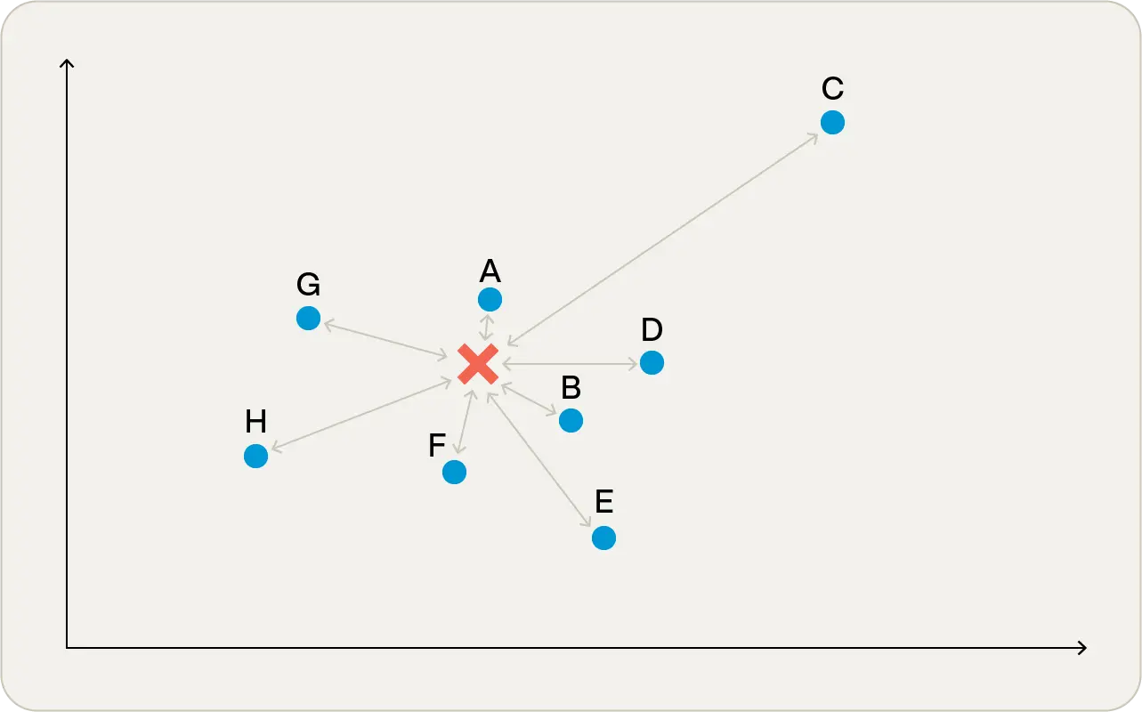
In Figure 1, you can see that point A is closest to the target point, and point C is furthest away. People tend to think of this as the obvious means of comparison as it’s what they’re used to seeing on 2-dimensional graphs. 

In fact, for low-dimensionality vector spaces, Euclidean distance normally yields the best results. The formula is quick and simple to implement, too:

This can be done in only a handful of lines of code, and the square root operation is the most computationally expensive. However, all that is required is the distance that is the smallest in the vector space. The actual value is largely irrelevant. So people often use “squared Euclidean" distance, which removes the expensive square root operation:

Cosine similarity

A different measure of “closeness” is cosine similarity. This is a little harder to explain. Imagine that you’re standing at the origin looking at the different vectors. Assume that no matter how close or far away the points are, all points are of equal size. So all you care about is the angle between the vectors:

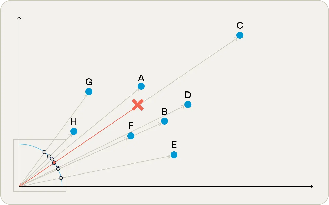
If you zoom in on the square near the origin in Figure 2, you can see the angles more clearly:

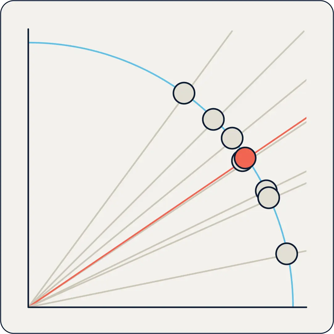
The red circle is the angle to the target vector, and you can see in the magnified view (Figure 3) that there is a point almost at the identical angle as our target vector. That point is actually point C, which oddly enough was the furthest away point using the Euclidean distance method!

So, the choice of algorithm used to compare vector similarity can make a huge difference to the result. Embedding models will often recommend a similarity algorithm they work best with, and there are some rules-of-thumb for selecting them. For example, as seen above, Euclidean distance works very well on low-dimensional vector spaces. Cosine similarity works well on high-dimensional vector spaces, so it is quite often used with embedding models used with LLMs.

The algorithm for cosine similarity is a bit more complex than Euclidean distance, but not significantly so. The mathematical definition is:

In this equation: 

x ᐧ y = dot product of x and y

||x|| = magnitude of x

Note that this algorithm gives a number in the range of -1 to 1, with higher numbers being more similar.

Results

As you now know, the similarity algorithm selected makes a difference in the results. Given that Euclidean distance works best for low-dimensionality vector spaces and the vectors in this example have just two dimensions, it is expected that this will yield better results. Applying the above formulae to all vectors compared to the desired target point gives:

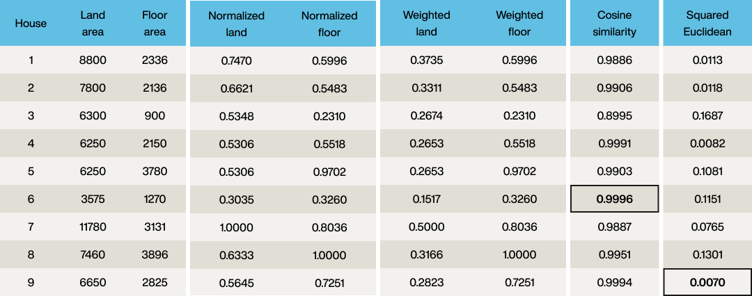
As can be seen, cosine similarity says property 6 is the closest match to the query vector, whereas squared Euclidean says property 9 is the best match. Which is correct? Well, the optimal property wanted a 2,500ft² floor area and 6,500ft² land area, and comparing these two properties shows:

• Property 6 has a 1,270ft² floor area and 3,575ft² land area

• Property 9 has a 2,825ft² floor area and 6,650ft² land area

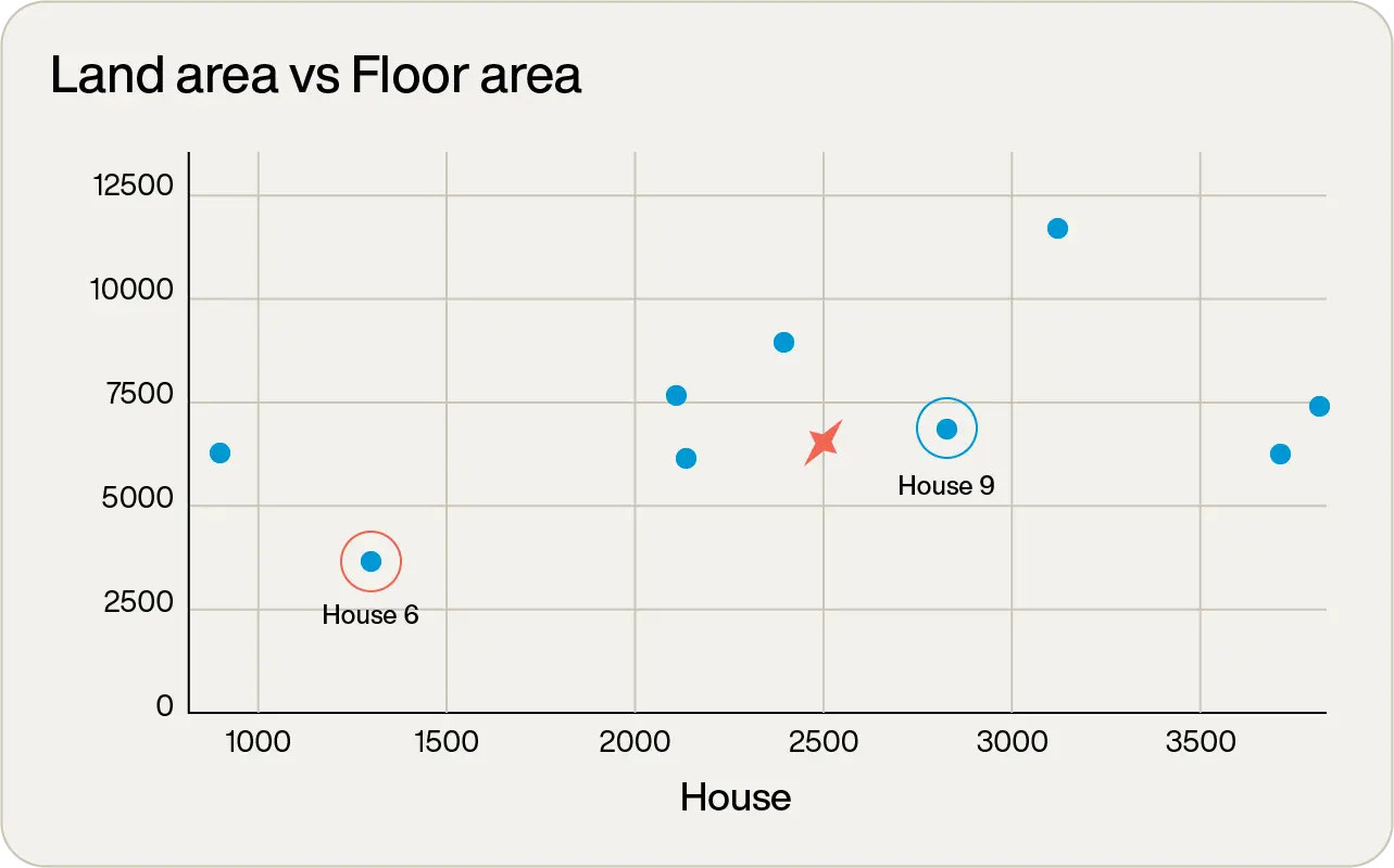
Clearly, property 9 is a way better match for our target property, which was expected as that was the result from the squared Euclidean algorithm.

Vector databases

By now you should have an understanding of vectors and similarity searches. This gives the tools to understand the use of a vector database. In a very simplistic view, a database has three main functions:

1. Store information, including both vectors and domain objects

2. Retrieve information

3. Perform a vector search with a chosen algorithm (Squared Euclidean, cosine similarity, etc.) against the database, retrieving the domain objects associated with the closest vectors to the passed vector. The number of domain objects to be returned is normally passed as a parameter to the search.

There are obviously many more complexities to a real vector database than this, including data security, data governance, audit controls as well as more advanced vector features like filtering, but this is a useful approximation of a simple vector database.

Naive implementation

These requirements of a basic vector database are so simple that an almost trivial implementation suggests itself. Storage (requirement 1) and retrieval (requirement 2) of information can be achieved with a dictionary-like structure, where the unique identifier of the business object is the key of the dictionary entry, and the other data, including the vector, is the value of the dictionary entry.

To perform the vector search (requirement 3), simply iterate through each domain object and the associated vector and then compute the similarity to the query vector. Keep the closest K domain objects, where K is the desired number of domain objects passed to the algorithm. Once all objects have been considered, return the set of closest objects.

This implementation is fairly similar to the process shown in the vector example above. It’s very simple, and it works well. 

However, it is not very efficient at scale. If you have hundreds or thousands of domain objects, iterating through all of them and calculating the similarity score is CPU intensive but should complete quickly. But what if there are a billion vectors? Or a trillion? This brute-force approach to a vector search would take an inordinate amount of time to complete at this sort of scale.

Index-based approach

Similar to most traditional databases, vector databases use indexes to help speed up the retrieval of vectors and their associated domain objects. However, the indexes typically are very different structures than are used in NoSQL or relational NoSQL databases. For the math gurus reading this, the indexes in a vector database are geometric indexes over an N-dimensional space, where N is the dimensions of the vector.

One of the most common approaches to indexing vector databases is the Hierarchical Navigable Small Worlds (HNSW) index. This graph-based algorithm has very fast retrieval times and high accuracy, even over large vector spaces. 

To understand how this index works at a high level, consider the earlier example. But now, instead of having nine properties to choose from, there are hundreds:

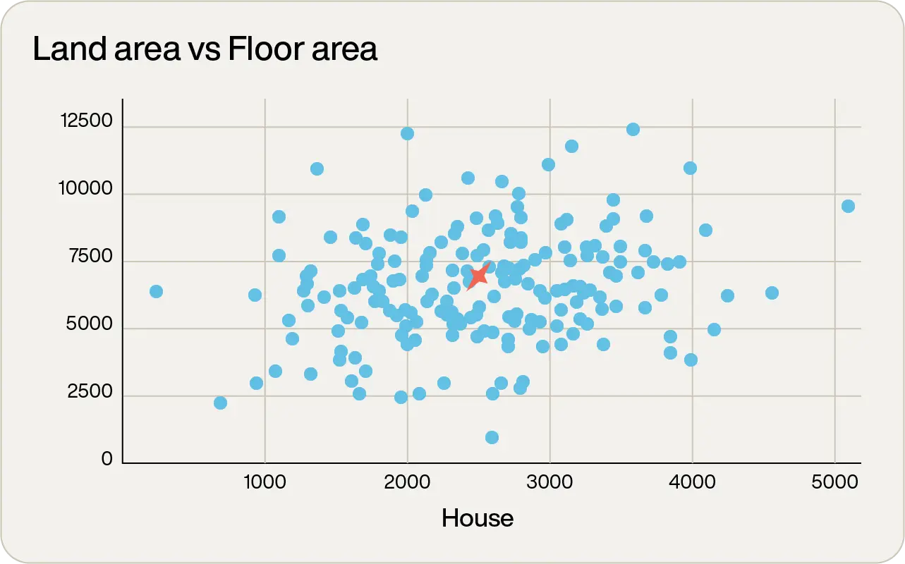
By simply inspecting the graph, there are some very obvious non-contenders. The lone one out on the far right with over 5,000tf² of floor space is way too big. There’s one on the far left with almost no floor area, which will be way too small. In fact, just by inspection, it is possible to visually categorize the areas:

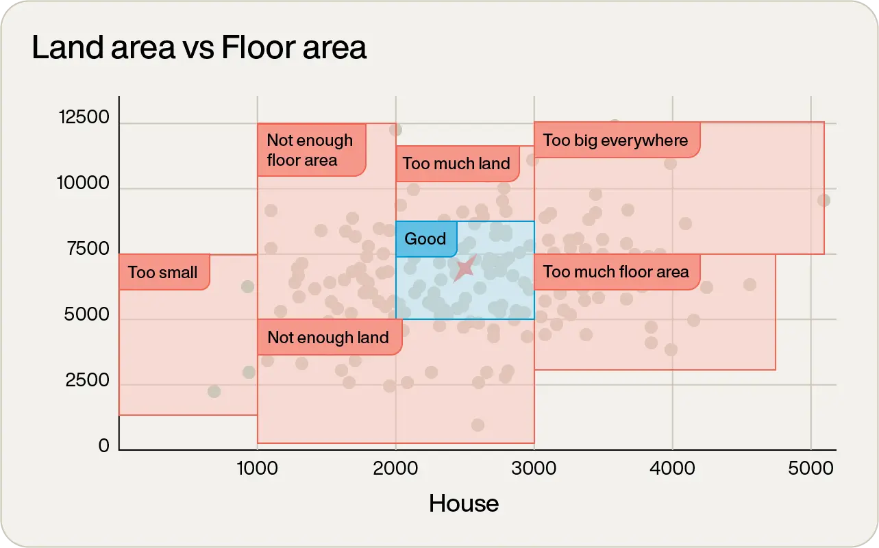
You could safely ignore anything that was not in the blue square in the middle. Great! In one simple inspection, the majority of the data points have been eliminated. So your next logical step would be to zoom in on the points in that area (pay attention to the scales on the axes in the following figure):

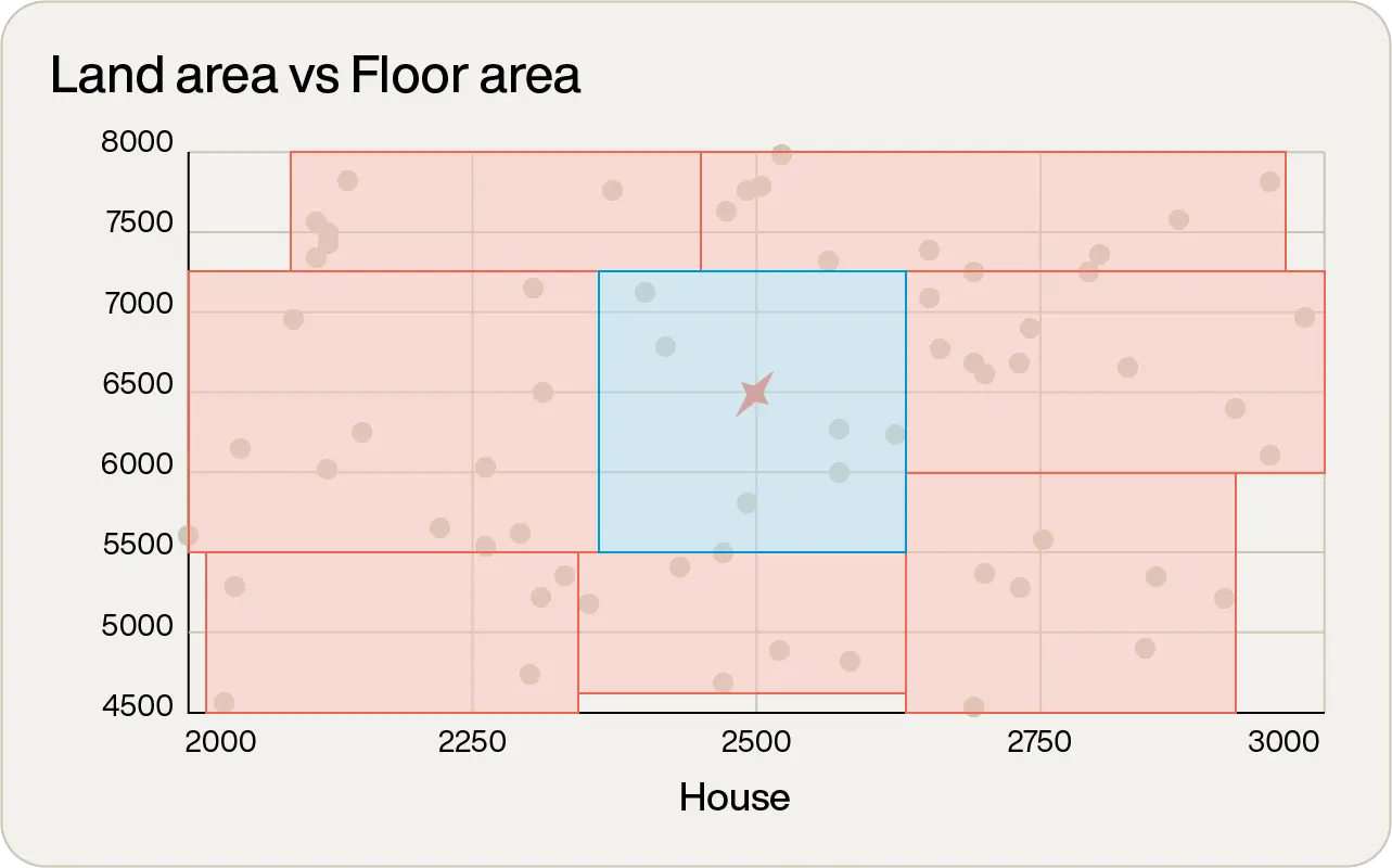
In this further magnified view, you would repeat the process: keep those points closest to the desired target and discard the rest. At this point you’re down to just eight data points to compare, which is small enough to perform brute force analysis on.

While this process seems intuitive, what you have just done is almost precisely how an HNSW index works. Start at a high level, with a few very large regions. Determine which region to focus on, drill down into that region, and then reapply the algorithm until the number of data points is small. 

Due to this hierarchical nature, you will often see images depicting HNSW similar to:

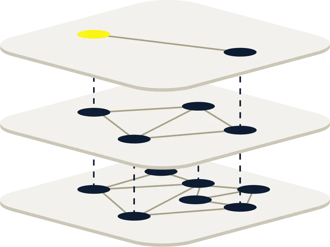
Note that the implementation of an HNSW index, while fairly simple to describe, is more complex to implement in an N-dimensional space. 

Why are vector databases important in AI?

The vector search algorithm is very useful in its own right. For example, consider trying to search a set of documents for a concept, as opposed to an exact search term. Each document might be embedded as a vector, or more likely, the documents might be broken into chunks and each chunk vector embedded. These vectors would be stored in a vector database. The search concept would also be embedded into the query vector and a similarity search conducted. This would yield similar vectors and hence the chunks of documents most pertinent to the query vector, and then the results could be displayed to the user.

This sort of “fuzzy matching” is still really a part of AI, as it typically requires advanced CNNs to translate the written language in the documents and search items into vector embeddings, a concept known as natural language processing (NLP).  

Another part of AI is generating humanly understandable responses, which would be in natural language written text, spoken words, generated images, or other formats. These responses typically come from LLMs as described earlier in this document, in a process known as generative AI.

LLMs are very complex pieces of software, typically requiring billions of calculations to form even a simple response. They are created using deep-learning techniques on very large volumes of data (referred to as a corpus in the AI community). This enables the LLMs to “know” things and give educated responses to appropriate inputs.

However, smart as these LLMs are, they suffer from several limitations:

• Stale training: The LLMs know only the information they were originally trained on, so anything that has happened or changed since that time cannot be queried.

• No domain-specific information: publicly available LLMs like OpenAI’s ChatGPT and Google’s Gemini (to name but a couple) are trained on publicly available data. This makes them unsuitable for querying domain-specific information like internal emails, confidential documents and so on, which was not publicly available at training time.

• Hallucinations: In some situations where the LLM has no information available to answer the query, it can create plausible-sounding but entirely fictional responses. These are referred to as hallucinations. 

All of these issues can be addressed by providing the LLM with contextual information in addition to the question that is being asked. This contextual information typically comes from a vector database having been queried with a semantic search. This process is known as retrieval augmented generation (RAG) as the LLM’s base training is augmented with the data retrieved from the vector database to help generate the response.

A pipeline for RAG would look something like:

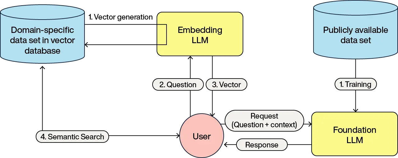
These steps should be familiar by now:

1. The vectors for the domain objects are generated using the embedding LLM, and these vectors are stored and associated with the domain objects

2. The user forms a query which gets submitted to the embedding LLM

3. The LLM returns the vector representing the query

4. The vector database returns the domain objects associated with the closest vectors

5. The user query is passed to the LLM along with the domain objects as the context and instructions on what the LLM is to do (called the prompt).

6. The LLM processes this information and forms a response back to the user.

Note that RAG is not the only solution to solving the LLM limitations. Another approach is using fine-tuning of the LLM, which provides more domain-specific information. Fine-tuning an LLM takes a pre-existing “foundational” LLM and feeds it additional annotated data along with expected results, allowing the LLM to learn.

Fine-tuning is particularly useful when the new details will only change infrequently. For example, fine-tuning can be particularly useful when the language of the domain is different from the language it was trained on. A foundational LLM trained in English would be far more useful in the legal domain if fine-tuned in legal language. 

In contrast, RAG is more useful when the data does change quickly, such as recommending stock market trades based on current conditions in a volatile market, or recommending products out of a product catalog in a recommendation system. One drawback to RAG is that the context provided to the LLM needs to be understood by the LLM before it is useful, resulting in billions of more computations and additional time. 

Fine-tuning LLMs and RAG are not mutually exclusive, and many situations can benefit from using both. For example, in a legal domain, fine-tuning would allow the LLM to understand and output legal jargon, and RAG would allow access to the latest court decisions to be ingested and analyzed for suitability in a particular case.

Explore vector search solutions with Aerospike

Vectors and vector databases are the backbone of many AI systems, providing relevant contextual information that can be used to prevent LLM hallucinations and enable responses based on the latest data. By converting structured or unstructured data into high-dimensional vectors through vector embedding models, vector databases provide easy search capabilities over a wide range of different source materials. Small-scale vector databases are trivially easy to implement; however, a scalable solution like Aerospike that uses advanced indexing techniques should be used for real-world vector retrieval, such as scale.