What is an in-memory database?

These days it seems common for database vendors to refer to themselves as “in-memory”. There is a proliferation of in-memory databases, in-memory data grids, and so on. But what does this really mean? The reference to “memory” implies speed, as memory is traditionally faster than storage, but are there sacrifices being made to other aspects of the database to accommodate this increased speed? This blog will outline types of memory, scalability factors, and performance results of different in-memory database architectures.

What types of memory are there?

There are various types of memory in modern computers. These will be discussed shortly, but it should be noted that there are tradeoffs between speed, cost, and capacity per device for the various types of memory. The fastest devices tend to require more transistors per bit stored, requiring more physical space and more cost to manufacture. Additionally, newer manufacturing technologies allow higher densities but at a premium cost. For example, at the time of writing this, a dual in-line memory module (DIMM) of 32GB of DDR5 DRAM operating at 4800MHz costs about $350 USD. 64GB with the same specs costs about $600 USD, but 128GB costs $2,600 USD, and 256GB about $9,500 USD. The 64GB modules offer the optimal price per GB, but with finite memory slots per motherboard, the higher capacity modules are sometimes needed for memory-intensive applications.

Random access memory

In classic computer architectures, memory meant exactly one thing – random access memory (RAM) which was attached to the computer’s motherboard and used to store temporary information. This information is non-persistent – when the computer is switched off, the information in that memory is lost. RAM is often divided into static RAM (SRAM) and dynamic RAM (DRAM). SRAM is typically faster but less dense and more expensive, so is typically used in things like CPU caches, whereas DRAM has a larger capacity, so it is commonly used for main memory in computers. Current SRAM caches are typically up to a few hundred MB, DRAM modules are in the range of 8-64GB for a comparison of densities.

Both SRAM and DRAM suffer from a common problem when used to store data in a database: they both require power to retain information. If the computer is turned off, all the information is lost, and this is clearly not ideal for a database. Modern distributed databases store multiple copies of each piece of information around a cluster of nodes, and many can re-replicate this data to other nodes if needed, but this still consumes network bandwidth and time.

Hence, the advent of non-volatile RAM or NVRAM. Early incarnations of these technologies either relied on battery backup to keep power to the RAM when power failed (not ideal) or used electrically erasable programmable read-only memory (EEPROM) technology. These were persistent (to a point, normally about 10 years) and could access information quickly (nanoseconds to a few microseconds), but writes were slower (up to several milliseconds), and they were destructive, so a typical device could only do 100,000 to 1,000,000 writes before it became unreliable. Additionally, the entire EEPROM had to be erased before any of it could be rewritten.

Solid state drives

EEPROMs, despite their drawbacks, formed the basis for a more recent class of memory – flash memory. Flash memory is persistent, available in high densities at relatively low cost, and forms the basis for USB sticks, SD cards used in digital cameras, and solid-state drives (SSDs). There are still drawbacks: they have finite write cycles and will “wear out” after having been written many times, and are not “byte-addressable.” Typically, a “page” is read or written at any time, and this is normally about 4KB.

SSDs are a form of memory, albeit persistent and slower than DRAM. A read from DRAM is around 60 nanoseconds or so; a read from an SSD is about 100 microseconds, so over a thousand times slower. However, SSDs are substantially more scalable than DRAM at a fraction of the cost. For example, at retail prices in early 2024, one terabyte of DRAM (8 x 128GB DIMMs) will set you back about $4,500 USD, whereas a fast NVMe SSD costs about $200 USD per terabyte. SSDs also have higher densities, with 12.8TB being common, and the largest SSDs commercially available are over 60TB! Of course, multiple SSDs can be placed on a single server too, making them convenient for fast, large-scale storage. Servers with over 100TB of SSD storage are easily purchasable in today’s market.

There are different classes of SSDs too. SATA SSDs are attached to the SATA bus which was introduced in the year 2000 to handle rotational drives. While many SATA SSDs can be attached to this bus, the design of the interface severely limits throughput, typically limiting maximum transfer rates to 600MB/s for a SATA III interface. In contrast NVMe SSDs typically sit in a PCIe slot on the computer’s motherboard and hence have direct access to CPU I/O lanes and have a theoretical maximum speed of 64,000MB/s! In both cases, the underlying storage is flash memory, but the difference in controllers means that NVMe SSDs transfer data substantially faster and have significantly shorter tail latencies than the SATA SSD equivalents. For the purposes of this article, both will be referred to as SSDs.

There are other classes on NVRAM, too, such as Intel’s Optane / 3d XPoint product, which is fast, byte-addressable, and very useful to address large, persistent storage requirements like databases. However, this technology is discontinued, so this discussion will focus on widely available technologies.

How scalable is an in-memory database?

The scalability of an in-memory database comes from its architecture. Most in-memory databases today distribute the data across multiple nodes in a cluster for resiliency so that the loss of a single node doesn’t bring down the whole database. However, in order for this to work, multiple copies of the data must be stored in the cluster. Many, but not all, distributed systems rely on quorum-based consensus algorithms like Raft, meaning that to tolerate a single node failure, they need three copies of the data.

As noted, DRAM is faster but substantially more expensive than SSDs. So if you’re looking for a moderate amount of data, a database that stores the information in DRAM is just fine.

What is “moderate”? Let’s say you want to store 1TB of unique data. If you’re using a quorum-based database, that requires three copies of the data, so you’re at 3TB of replicated data. That doesn’t allow for overhead due to fragmentation, compactions, etc, so in reality, you probably require closer to 5-6TB of DRAM. Thus you’re probably in the range of about $25,000 USD for the memory costs alone for the cluster. Then you have to add in CPUs, NICs, power supplies, rack space, switches, etc. DIMMs scale up to a point, but as noted earlier, there is an exponential cost growth of larger-sized DIMMs as well as physical limits on the number of modules supported per motherboard. Hence, the point of requiring scale-out is reached fairly quickly, resulting in larger clusters and increased hardware costs.

As the unique data grows, so does your cost. 40TB of unique data would cost well over $1M USD just in hardware alone.

Can SSDs help scale in-memory databases?

SSDs offer far better scalability compared to DRAM. Densities are higher, and more can be used per machine, especially with the use of fast NVMe riser boards to allow sharing of CPU I/O lanes. However, they are slower, and unless the database is explicitly architected from the ground up to use the SSD characteristics, they can become a significant performance bottleneck. Let’s look at one in-memory database designed from the ground up to use SSDs in conjunction with DRAM, providing a great combination of performance and scalability – Aerospike.

Read path

Consider the illustration below when reading a record from the client:

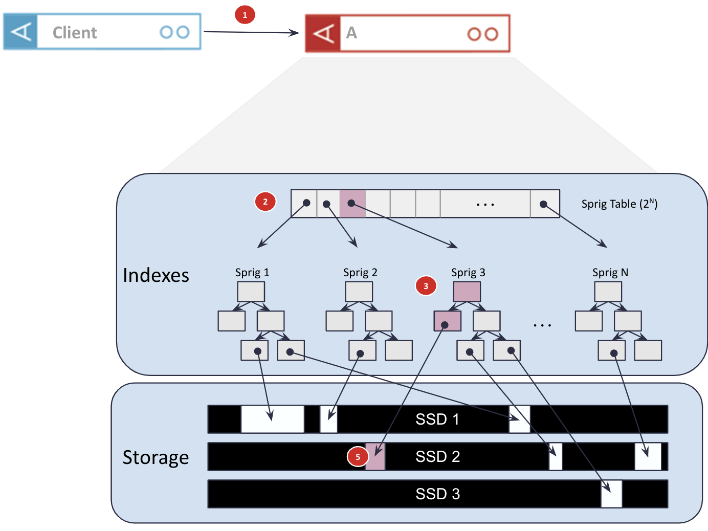
Figure 1: Aerospike’s read path from the client to storage.

The numbers shown in Figure 1 show the following points in the read path:

1. The client application is typically on a different machine than the database nodes, so it needs to do a network hop to the node that owns the data. In Aerospike’s case, this is a single network hop through use of a constant hashing algorithm rather than having to bounce off a coordinator node of any description.

2. On reaching that node, a hash table is consulted to determine which primary index sub-tree (“sprig”) holds the desired information. This hash table typically lives in DRAM but is reasonably small, typically a few megabytes per node.

3. This sprig is traversed to find where the data lives on SSDs and the size of that data. The sprig is a balanced red-black tree, so this traversal has O(log2 N), where N is the number of records in that sprig. These sprigs also typically reside in DRAM for fast traversal.

4. The data is read from the location on the SSD and returned to the client.

There are other optimizations Aerospike takes to make this quick, the most notable is the lack of a file system on the SSDs. The disks are used in raw or block mode, providing direct access to any location on the drive with no file system penalties.

Write path

Writes are more complex as SSDs, like their EEPROM ancestors, are typically not fast at writing to storage, and writes are also destructive, causing wear on the SSD. Hence a record should be written as few times as possible to lower the “write amplification” – the number of times a single write is written.

This is another advantage of not having a file system on the SSD. A file system can move data around under certain conditions, causing more write amplification. Block mode writes do not.

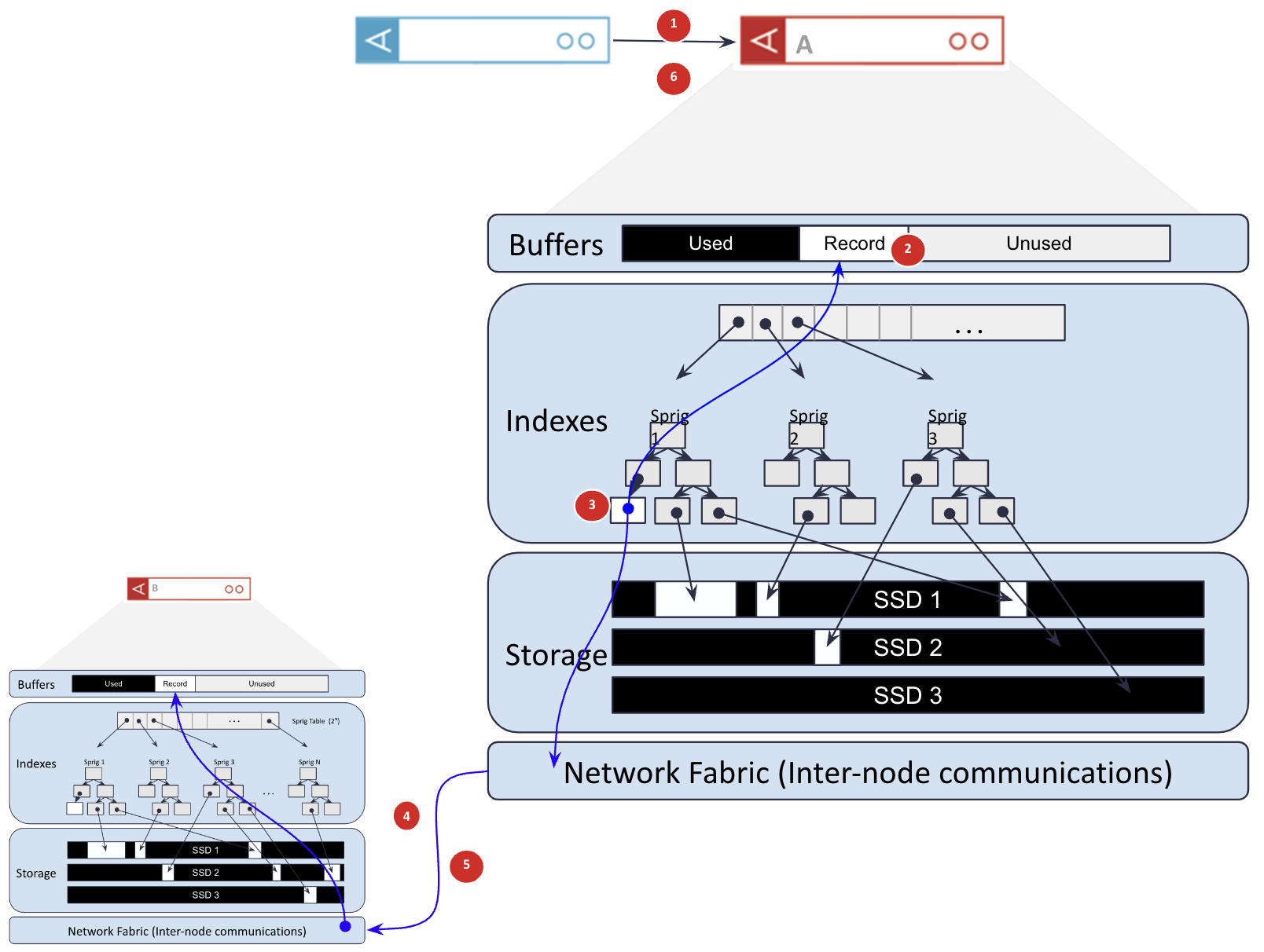
Figure 2: Aerospike’s write path from client to storage.

In the write path shown in Figure 2, the numbers refer to the following steps:

1. The client does a single network hop to the node that owns the piece of data being written.

2. Instead of writing directly to the SSD, the write is written into a DRAM write buffer. This buffer is small, 8MB or less depending on the configuration used.

3. The primary index entry for that record is either created (for an insert) or amended (for an update) to point to the memory buffer.

4. The data is replicated to one or more other nodes over the network.

5. The replica node(s) respond to the master node once they have stored the information in their write buffer.

6. Now the master and all replicas have a copy of the record, the write is acknowledged to the client.

7. At some point later, the write buffer is flushed to storage. This occurs either when the write buffer is full or a second has elapsed, whichever comes first.

Performance differences between DRAM and SSDs

DRAM performance is better than SSD, but let’s look at the relative performance of pure in-memory versus this solution. On the read path, the round trip network hop from the client to the database server and back again takes about 100 microseconds. Let’s assume that retrieving the information from memory takes negligible time – not necessarily a valid assumption, but it gives best-case numbers for DRAM performance. So, round-trip time for the client to read a record from DRAM takes about 100 microseconds. A read from a good quality SSD is also about 100 microseconds, so with the 100 microseconds network hop, the read with this architecture – off storage, not out of memory – is about 200 microseconds, round trip. The nice thing about this architecture is that reading any record will have approximately the same latency, as there is no concept of “cached data” and hence no cache misses. This gives a very predictable, flat-line latency.

With writes, this architecture writes to memory and does not wait for the flush to SSD, which is the slow part of using SSDs as storage. So writes are effectively done at memory speed, either using DRAM as storage or SSDs as storage. In both cases, there are multiple network hops – one from the client to the master and one from the master to the replica. If there are multiple replicas, these writes are done in parallel, so the total elapsed time is similar.

Note that Aerospike can guarantee strong consistency with just two copies of data; it is not based on a quorum architecture. This can offer substantial savings on hardware compared to the three copies of data needed for quorum-based architectures.

Reading is about 100 microseconds slower with storage on SSD than out of DRAM and writes are fairly similar between the two architectures. However, DRAM is limited in practice to 10’s of TB, whereas the SSD implementation can scale to multiple petabytes of data.

Cost differences between DRAM and SSDs

As a comparison on cost, consider storing 50TB of unique data in a pure DRAM-based database compared to a database like Aerospike, which uses SSDs in conjunction with DRAM. Assuming both databases store three copies of data (not necessarily true in Aerospike’s case), the amount of data stored is about 150TB. There is overhead due to data fragmentation, room needed for compactions, metadata level overhead, etc., so it’s reasonable to assume for both databases that ~250TB of storage is needed.

With a pure DRAM-based database, the DRAM costs will likely be around $4,500 USD x 250 or $1,125,000 USD. Given the practical densities of DRAM, the cluster size would probably be in the hundreds of nodes, meaning large costs for CPUs, NICs, switches, rack space, cooling, power, management costs, maintenance costs, etc.

With an SSD-optimized database like Aerospike, each node could easily store 25TB of data on SSDs, with 2 x 12.8TB drives per node. The drives would likely cost around $5,000 USD (total), so fully loaded with, say, 512GB DRAM, CPUs, power supplies, etc, each node would probably be around $15,000. Only 10 nodes are needed in this scenario, for a total cost of around $150,000 for the cluster. This is an 85% reduction in hardware costs, and that is considering just the DRAM costs of the DRAM-based database, not the fully loaded costs, against the fully-loaded costs of the SSD-optimized solution.

(Note: The numbers here represent the retail costs available on the internet. Different vendors will offer different prices based on the level of support, reliability, and so on. These numbers should be considered indicative of the cost ratio between the two solutions, not what specific hardware will cost)

An in-memory database optimized for scale and cost

In-memory databases that use DRAM as storage offer incredible performance but have limited scalability in terms of data storage. However, the term in-memory also can include SSDs, and databases like Aerospike, which are optimized from the ground up to use SSDs, are also a class of in-memory database but offer substantial improvements on scalability for very little performance cost. Mixing DRAM and SSDs to optimally utilize the characteristics of each memory class like Aerospike does offers the best of both worlds, giving very fast access and almost unlimited scalability at a fraction of the cost of other solutions at scale.