A developer’s introduction to graph databases

Get ready to deploy a real-world dataset on Aerospike Graph and execute queries in just a few minutes.

Ready to dive into new realms of graph technology and discover fascinating insights with each click? Whether you're a curious beginner or a seasoned graph explorer searching for fresh perspectives, this blog is meant for you.

Aerospike Graph at a glance

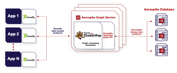
Aerospike Graph leverages Apache TinkerPop, an open-source graph computing framework, and Gremlin, a graph traversal language. In other words, Gremlin is a query language, like SQL, for traversing and manipulating graph-structured data. Using Gremlin, you can explore specific graph traversal sequences known as traversals. Our post, Aerospike and gdotv partnership delivers rich graph data visualization goes further into the capabilities at your disposal when using a Gremlin IDE.

Aerospike Graph is built on top of the Aerospike Database, a high-performance, scalable, and reliable database engine. Aerospike Graph can build and operate large-scale graph applications across many use cases, including customer 360 and fraud prevention, among others.

Working with graph data

In this example, we examine various queries that explore a graph which contains a model of the worldwide air route network. The air-routes graph schema (see figure below) models a transportation network for air routes. It represents airports, countries, and continents as vertices and flight routes (i.e., routes) and continents or countries (i.e., the airport's location) as edges between the vertices. Each vertex (e.g., airport) has properties such as an airport code, name, location (latitude and longitude), and time zone. Similarly, edges (routes) can have properties such as distance between airports.

The schema includes the following elements:

1. Airport vertex: Represents an airport in the transportation network. It has properties such as:

   • code: The unique code assigned to the airport.

   • name: The name of the airport.

   • location: The geographical coordinates of the airport (latitude and longitude).

   • timezone: The time zone of the airport.

2. Route edge: Represents a flight route between two airports. It has properties such as:

   • airline: The name of the airline operating the flight.

   • distance: The distance between the airports.

Additionally, the schema could include other optional properties or additional vertex and edge types to represent more complex relationships, such as intermediate stops or connecting flights. The specific implementation of the graph schema may vary depending on the use case and your requirements. The remainder of the blog describes the software prerequisites, the Docker images you need, how to connect and load the data, and how to execute some queries.

Why Docker containers? If you are a developer working on multiple machines, each time you switch a machine, you need to set up and configure the database separately.

Using Aerospike Database and Aerospike Graph inside a Docker container, you can quickly spin up a sandbox environment and focus on actual development rather than infrastructure setup. The same is true for the production environment.

1. Software prerequisites

As usual, there are a few prerequisites that need to be taken care of before you begin. Following is a list of the software used to run this JupyterLab Notebook.

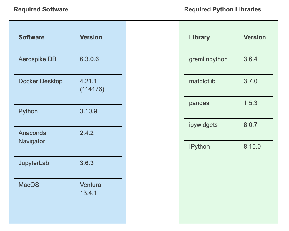
The next section provides the steps to download the Docker images and launch the Graph Service and Database containers.

Download Aerospike software

Once you have Docker installed, the simplest way to get up and running is to pull the Aerospike images from the Docker hub repository. In a terminal window, execute the following pull commands:

docker pull aerospike/aerospike-serverdocker
docker pull aerospike/aerospike-graph-servicedocker

You’ll also need a trial license key for the Aerospike Graph Service. Get started by downloading a free trial.

If you would like detailed steps on how to start the containers, take a look at the Aerospike Graph Using Docker documentation. However, the steps below should be enough to get you started.

1. Set an environment variable with the license key (aka, Feature Key). export FEATKEY=$(base64 -i /<YOUR_PATH>/<YOUR_FEATURE_KEY.conf>)

For example:

export FEATKEY=$(base64 -i /Users/Shared/setup/as_featurekey.conf)

2. Launch the database container.

docker run -d -e "FEATURES=$FEATKEY" -e "FEATURE_KEY_FILE=env-b64:FEATURES" --name as_database -p 3000-3002:3000-3002 aerospike/aerospike-server-enterprise

3. Launch the graph service.

docker run -p8182:8182 --name as_graph -v <PATH_TO_YOUR_SHARED_DIR>:/opt/aerospike/etc/sampledata -e aerospike.client.namespace="test" -e aerospike.client.host="172.17.0.2:3000" -e aerospike.graph.index.vertex.label.enabled=true aerospike/aerospike-graph-service

For example:

docker run -p8182:8182 --name as_graph -v /Users/Shared/data/docker-bulk-load:/opt/aerospike/etc/sampledata -e aerospike.client.namespace="test" -e aerospike.client.host="172.17.0.2:3000" -e aerospike.graph.index.vertex.label.enabled=true aerospike/aerospike-graph-service

NOTE: The -v option allows you to bind a directory in your host operating system to a directory inside the Docker container. Make sure the air-routes-latest.graphml has been copied to the shared directory <PATH_TO_YOUR_SHARED_DIR> in the command above. You can download the air-routes-latest.graphml file form here.

Importing Python modules

Execute the following cell to import the packages you need. You might need to install them first using the pip command.

from importlib.metadata import version
from pandas.plotting import table
from ipywidgets import interact
from IPython.display import Markdown as md, display, HTML
from IPython.display import display_markdown
from gremlin_python.process.traversal import IO
from gremlin_python.process.anonymous_traversal import traversal
from gremlin_python.driver.driver_remote_connection import DriverRemoteConnection
from gremlin_python.process.graph_traversal import GraphTraversalSource, __
from gremlin_python.process.traversal import Barrier, Bindings, Cardinality, Column, Direction, Operator, Order, P, Pop, Scope, T, WithOptions

import matplotlib.pyplot as plt
import nest_asyncio
import networkx as nx
import ipycytoscape
import jugri
import pandas as pd
import re

nest_asyncio.apply()

2. Connect to the graph service and load the air-route data

To traverse the vertices and edges in the graph, you must spawn a traversal object:

g = traversal().withRemote(DriverRemoteConnection('ws://0.0.0.0:8182/gremlin','g'))

The above Gremlin query represents a simple pattern for creating a traversal object using a remote connection. Here is the breakdown of each part:

• g: This variable represents a reference to the traversal object. It allows you to build and execute queries on the graph database.

• traversal(): This function creates a new traversal object. It is the entry point for executing queries in Gremlin.

• withRemote(DriverRemoteConnection('ws://0.0.0.0:8182/gremlin','g')): This command configures the traversal object to use a remote connection to communicate with the Aerospike database. The DriverRemoteConnection class is used to establish the connection.

  • ws://0.0.0.0:8182/gremlin: This parameter specifies the WebSocket endpoint URL of the server hosting the graph database.

  • g: This parameter represents the specific traversal source on the server.

By executing this query, you can perform various graph database operations using the 'g' traversal object linked to the specified remote connection.

The next step is to populate the graph. The air-routes data should already be in the Aerospike Graph Service container. The file name is air-routes-latest.graphml and should be in the /opt/aerospike/etc/sampledata directory.

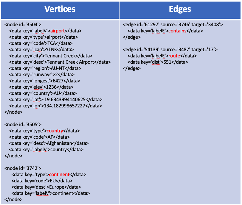
The file is in GraphML format. GraphML is an XML-based file format for graphs shown in the table below. On the left column, there is one entry (a record) for each one of the vertices in the graph schema, namely continent, airport, and county. The column on the right shows the format for edges.

Populate the graph (vertices and edges)

The following cell executes two statements. The first one drops all data in the graph. The second one loads the data using the io() step. The evaluationTimeout parameter prevents the loading operation from timing out when running for extended periods. In the following example, the timeout is set to 5 minutes in milliseconds (even though it takes a couple of seconds to load the air-routes data). You can adjust it as necessary.

g.V().drop().iterate()

g.with_("evaluationTimeout", 5 * 60 * 1000)\
  .io("/opt/aerospike/etc/sampledata/air-routes-latest.graphml")\
  .with_(IO.reader, IO.graphml)\
  .read()\
  .toList()

Once the data is loaded you can get a count of vertices and edges. To get a count of the total number of vertices loaded, execute the following statement:

g.V()
  .label()
    .groupCount()
  .toList()

• g.V(): This step retrieves all the vertices in the graph.

• .label(): This step extracts the label of each vertex.

• .groupCount(): This step counts the occurrences of each unique label and creates a map with the label as the key and the count as a value.

• .toList(): This step converts the map into a list, which can be returned as the final result of the Gremlin query.

NOTE: I am using Pandas data frames to capture the output of the queries and display the result either in tabular form or as a matplotlib chart.

v_cnt = pd.DataFrame.from_dict(g.V().label().groupCount().toList()).T   # .T to Transpose the dataframe
v_cnt.reset_index(inplace=True)
v_cnt.columns = ['vertex name','count']

To get the number of edges loaded, replace the g.V() step for g.E().

g.E()
  .label()
    .groupCount()
  .toList()

e_cnt = pd.DataFrame.from_dict(g.E().label().groupCount().toList()).T   # .T to Transpose the dataframe
e_cnt.reset_index(inplace=True)
e_cnt.columns = ['edge name','count']

The cell below uses matplotlib to display the counts as a bar chart.

 display_markdown(f'''## Total Number of Vertices: {v_cnt['count'].sum()}; Total Number of Edges: {e_cnt['count'].sum()}''', raw=True)
fig, axes = plt.subplots(nrows=1, ncols=2, figsize=(20,5))
ax1 = v_cnt.sort_values(by = 'count', ascending=False,).plot.bar(ax=axes[0], title='Vertex Counts', x='vertex name', rot=50, color = 'red')
ax1.set_ylabel("vertices Count")
ax1.bar_label(ax1.containers[0])
ax2 = e_cnt.sort_values(by = 'count', ascending=False,).plot.bar(ax=axes[1], title='Edge Counts',x='edge name', rot=50, color = 'green')
ax2.set_ylabel("edges Count")
ax2.bar_label(ax2.containers[0])
plt.show()

After executing the above code you will get a count of vertices and edges in the graph.

Total number of vertices: 3749; Total number of edges: 57645

3. Traverse the graph data

The last section of this blog presents some examples of Gremlin traversals that take advantage of the speed of the Aerospike Database.

If you are new to Gremlin, this document, PRACTICAL GREMLIN: An Apache TinkerPop Tutorial, is a great place to start. I've added comments to make the queries easy to understand.

Query 1: Retrieve all columns for the airport with code 'AUS' (Austin)

The first query looks at all the data in the graph and filters vertices that have the 'AUS' airport code.

g.V()
  .has('code','AUS')
    .valueMap()
  .next()

• g.V(): The vertex set of all the vertices in the graph.

• .has('code','AUS'): Filtered by vertices with code = 'AUS'.

• .valueMap(): Projects the result as a key value map of all the vertex properties.

• .next(): Returns the final result set of the query.

display(pd.DataFrame(g.V().has('code','AUS').valueMap().next()))

Query 2: Display a pie chart of the ten top countries with the greatest number of airports

The next query demonstrates a count aggregation. It filters all the vertices labeled 'airport' and counts the number of airports by country.

g.V()
  .hasLabel('airport')
    .groupCount().by('country')
  .next()

• .hasLabel('airport'): Create a vertex set of all the vertices with the vertex label equal to 'airport'.

• .groupCount().by('country'): Group and count all occurrences of airports by country.

df = pd.DataFrame(g.V().hasLabel('airport').groupCount().by('country').next(), index=['Airports']).T
df.reset_index(inplace=True)
df.rename(columns = {'index':'Country'}, inplace = True)
srt_temp = df.sort_values(by = 'Airports', ascending=False)
not_top_ten = len(srt_temp) - 9
not_top_ten_sum = srt_temp.tail(not_top_ten).sum()
srt_top = srt_temp.head(9)
new_record = pd.DataFrame([{'Country':'Other', 'Airports':not_top_ten}])
df = pd.concat([srt_top, new_record], ignore_index=True)
df.sort_values(by = 'Airports', ascending=False, inplace=True)

plt.figure(figsize=(16,8))
ax1 = plt.subplot(121, aspect='equal')
df.plot(kind='pie', y = 'Airports', ax=ax1, autopct='%1.1f%%', 
 startangle=90, shadow=False, labels=df['Country'], legend = False, fontsize=10)

ax2 = plt.subplot(122)
plt.axis('off')
tbl = table(ax2, df, loc='center')
tbl.auto_set_font_size(True)
tbl.set_fontsize(10)
plt.show()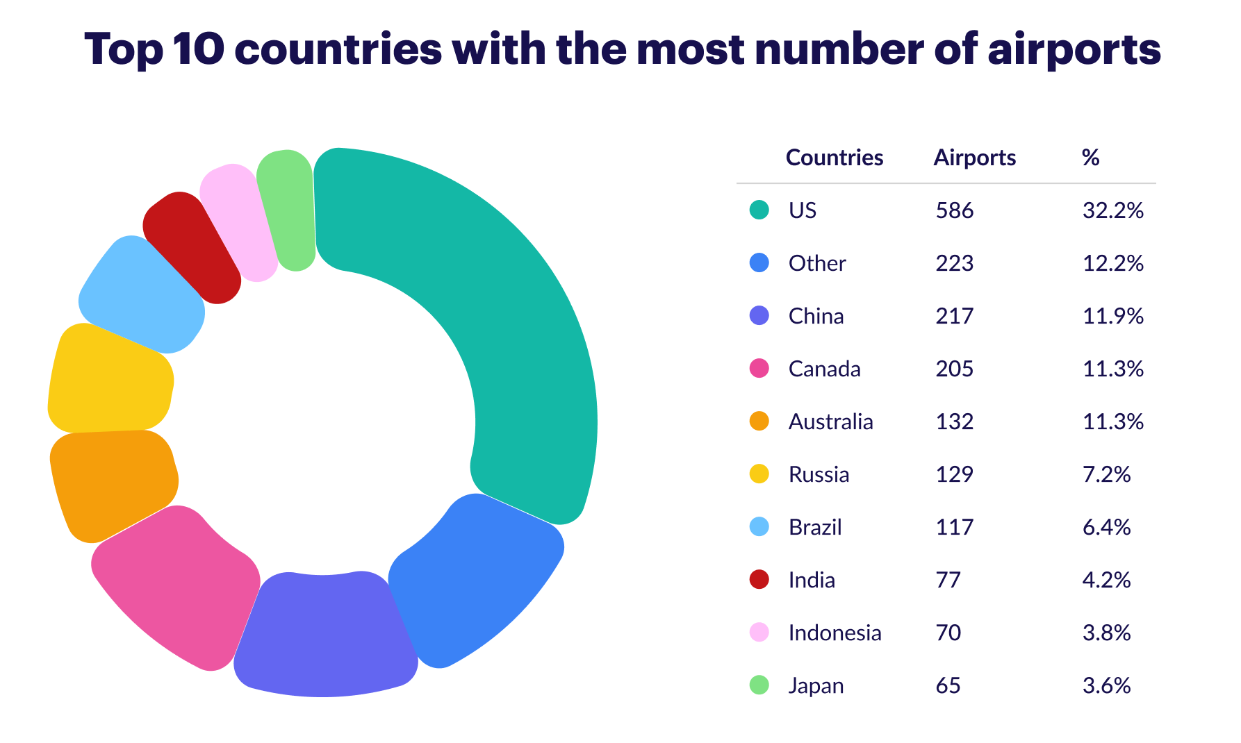

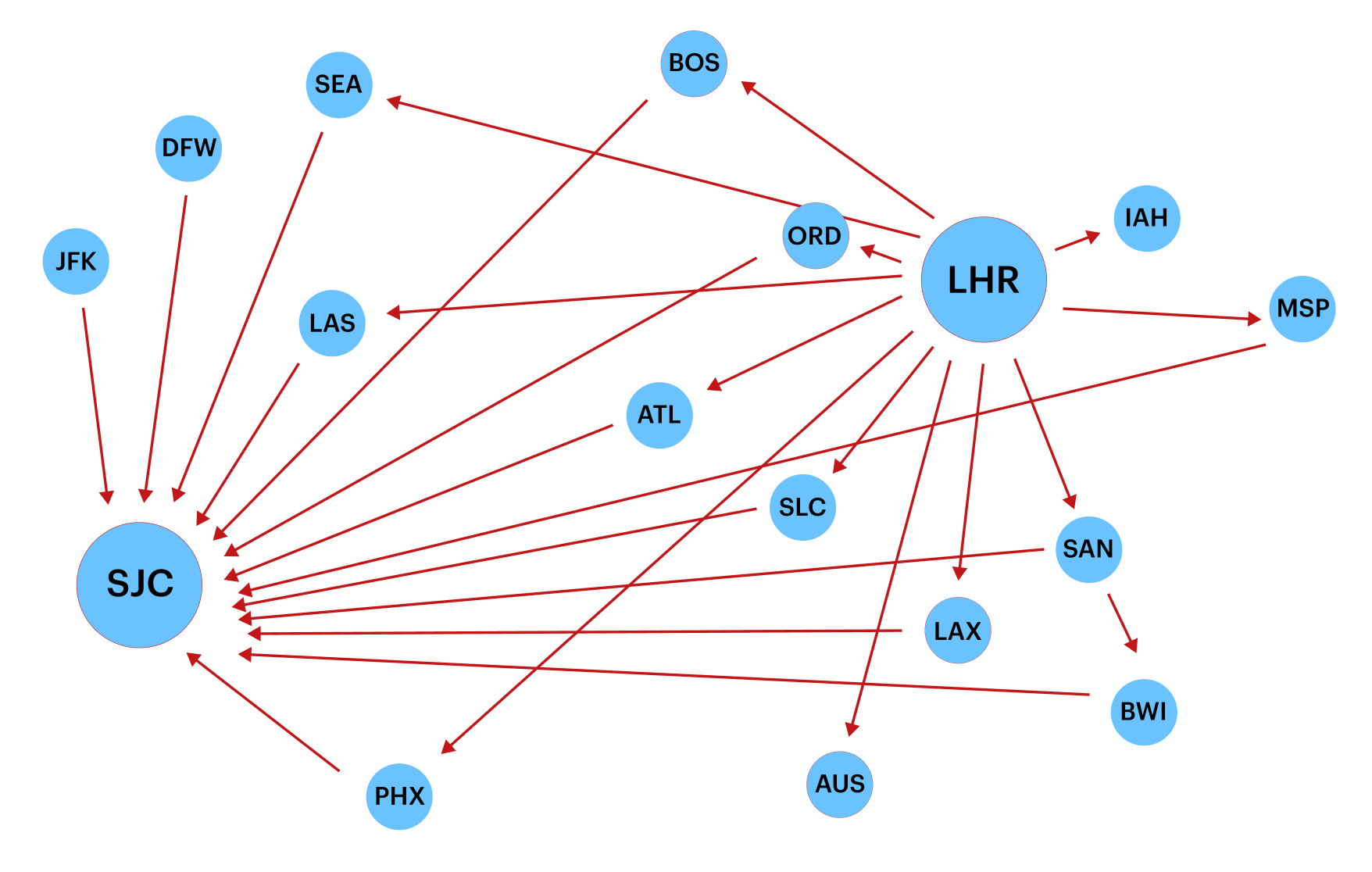
Query 3: Show possible routes from London to San Jose with one stop

This query limits the number of vertices returned using the limit() step.

g.V()
  .has('airport','code','LHR')
    .out().out()
      .has('code','SJC')
      .limit(15)
    .path()
    .by('code')
  .toList()

• .has('airport','code','LHR'): Filters the vertices by those with the property 'airport' and 'code' value equal to 'LHR' (London Heathrow Airport).

• .out().out(): Traverses two steps out from the previous filtered vertices. This means it retrieves vertices that are connected by edges going out two times from the 'LHR' vertex. These vertices represent flights departing from London Heathrow Airport, possibly making a stopover at another airport.

• .has('code','SJC'): Filters the vertices retrieved in the previous step by those with the property 'code' equal to 'SJC' (San Jose International Airport).

• .limit(15): Limits the result to only return a maximum of 15 vertices.

• .path().by('code'): Retrieves the paths taken to reach the filtered vertices represented by the 'code' property of each vertex. This means it returns the flight routes from London Heathrow Airport to San Jose International Airport.

display(HTML("<style>.container { width:100% !important; }</style>"))
df = pd.DataFrame(g.V().has('airport','code','LHR').out().out().has('code','SJC').limit(15).path().by('code').toList())
df.rename(columns = {df.columns[0]:'Path'}, inplace = True)
legs = pd.DataFrame(columns=['Source_Airport', 'Dest_Airport'])
df = df.astype('str')
for index, row in df.iterrows():
    s = re.search(r"path\[(.*), (.*), (.*)\]", str(row))
    legs.loc[len(legs)] = [s.group(1),s.group(2)]
    legs.loc[len(legs)] = [s.group(2), s.group(3)]
df1 = pd.DataFrame(legs['Source_Airport'].unique(), columns = ['Airport'])
df2 = pd.DataFrame(legs['Dest_Airport'].unique(), columns = ['Airport'])
vertices = pd.concat([df1, df2])
vertices = pd.DataFrame(vertices['Airport'].unique(), columns = ['Airport'])
vertices_list =[(v, {"label": v}) for v in vertices.Airport.values.tolist()]
NX_graph = nx.DiGraph()
NX_graph.add_nodes_from(vertices_list)
NX_graph.add_edges_from(legs.values.tolist())

# Display the first 5 rows only in tabular form
display(legs.head(5))
nx.draw_networkx(NX_graph, node_size=1000, font_color='#FFF', node_color='#b20b00', pos=nx.spring_layout(NX_graph), with_labels=True)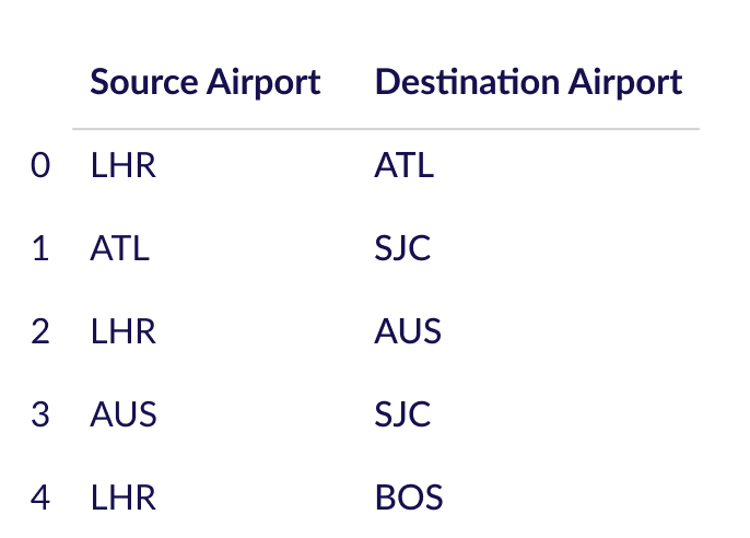

Query 4: Return a map where the keys are the continent codes and the values are the number of airports in that continent

In this next query, use a child traversal that spawns anonymously from __. Usually, the function that gets this traversal will connect it to the previous traversal, as depicted in the following:

g.V()
  .hasLabel('continent')
    .group()
      .by('code')
      .by(__.out().count())
  .next()

• .hasLabel('continent'): This filters the vertices to only include those with the label 'continent'.

• .group(): This function groups the filtered vertices.

• .by('code'): This specifies that the grouping key will be 'code' property of the vertices.

• .by(__.out().count()): This specifies that the value for each group will be the count of outgoing edges from each vertex.

m = g.V().hasLabel('continent').group().by('code').by(__.out().count()).next()

fig,pie1 = plt.subplots()
pie1.pie(m.values() \
        ,labels=m.keys() \
        ,autopct='%1.1f%%'\
        ,shadow=True \
        ,startangle=90 \
        ,explode=(0,0,0.1,0,0,0,0))
pie1.axis('equal')  

plt.show()

Query 5: Find the number of international and domestic flights with one stop from SFO

The following query introduces four more steps. Namely, Project: “fold and unfold.”

g.V()
  .has("code", "SFO")
    .out().out()
      .dedup()
      .fold()
  .project("International Flights From SFO", "Domestic Flights From SFO")
    .by(__.unfold().count())
    .by(__.unfold()
      .has("country", "US")
      .count())
  .next()

• .dedup(): Use the dedup step to remove duplicates from a result.

• .fold(): Gathers all elements in the stream to that point and reduces them to a List.

• .unfold(): Does the opposite, taking a List and unrolling it to its individual items and placing each back in the stream.

• .project(): Similar to SQL project, that is, which properties we want to pick for display.

display_markdown(f''' ### {
g.V().has("code", "SFO").out().out().dedup().fold().project("International Flights From SFO", "Domestic Flights From SFO").by(__.unfold().count()).by(__.unfold().has("country", "US").count()).next()
}''', raw=True)

{'International Flights From SFO': 1904, 'Domestic Flights From SFO': 455}

Start exploring the world of graph

In this blog, I have shared a high-level view of the different layers of the Aerospike Graph Service and how those layers interoperate from the application layer to the database layer. I have also looked at the advantage of using the python_gremlin library to execute queries against the Aerospike database, which helps simplify the application development.

Aerospike Graph leverages open-source components, including the TinkerPop graph engine and the Gremlin graph query language. The current release initially addresses OLTP workloads, such as fraud detection and identity authentication, with OLAP functionality in the future. You can use it with many different programming languages; Python and Java are just two examples. Choose the language that works best for you.

I suggest you try it out. Get the most out of your data with an Aerospike Graph 60-day free trial.